Chapter 5: Give It a Market — Liquidity on Raydium
How Automated Market Makers Turn Tokens into Tradeable Assets
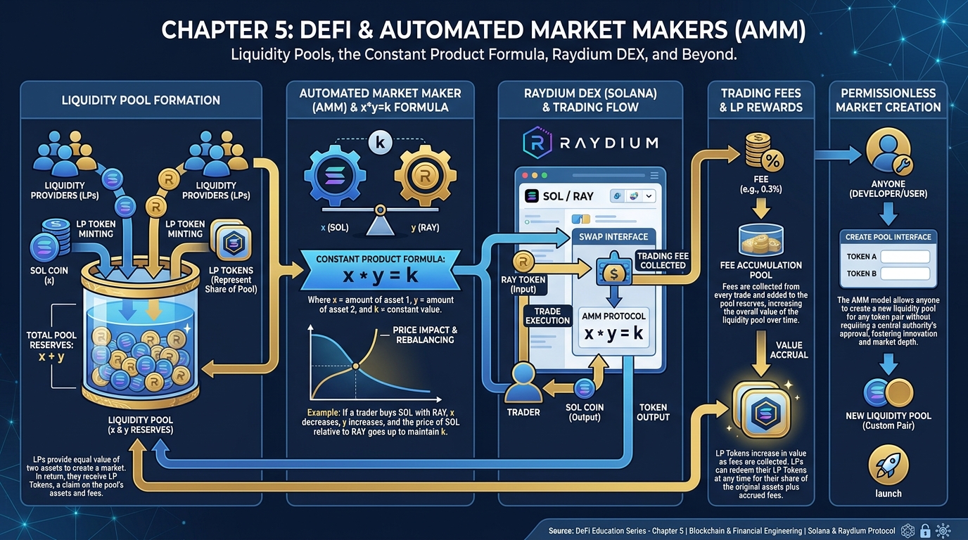
Figure 1:Chapter 5 at a glance: Liquidity pools, automated market makers, the x·y=k formula, and the Raydium interface — everything you need to open a market for your token.
A baseball card locked in a drawer is not an asset. It has no price. Nobody can buy it. You cannot liquidate it in an emergency or profit from its rising fame. It is a trophy with no market. Your token is in that drawer right now.
You minted it. You launched it. Maybe you even designed an elegant tokenomics model in Chapter 4. But until someone other than you can buy and sell it at any moment, it remains a specimen in a jar — interesting, but inert. This chapter is about building the store. Except this store has no employees, never closes, runs on math, and sets its own prices in real time.
Welcome to liquidity on Raydium.
▶ Deep Dive: Introduction to DeFi (31 min)
1What Liquidity Actually Means
The word “liquidity” sounds like finance jargon, but the idea is almost physical. Imagine trying to sell a rare piece of art versus selling a dollar bill. The dollar bill sells instantly at a known price. The painting might take months, and the final price is uncertain. The dollar bill is liquid. The painting is illiquid.
For any asset — a stock, a currency, a token — liquidity has two components: depth (how much can be bought or sold without moving the price significantly) and immediacy (how fast a transaction can complete). A liquid market has both. An illiquid market has neither.
Why does this matter? Markets without liquidity die. Here is the death spiral: without liquidity, no serious buyer shows up because the price is too unpredictable. Without buyers, no seller wants to hold the asset. Without sellers, there is nothing to buy. The asset goes to zero not because it was worthless, but because nobody could agree on a price in real time.
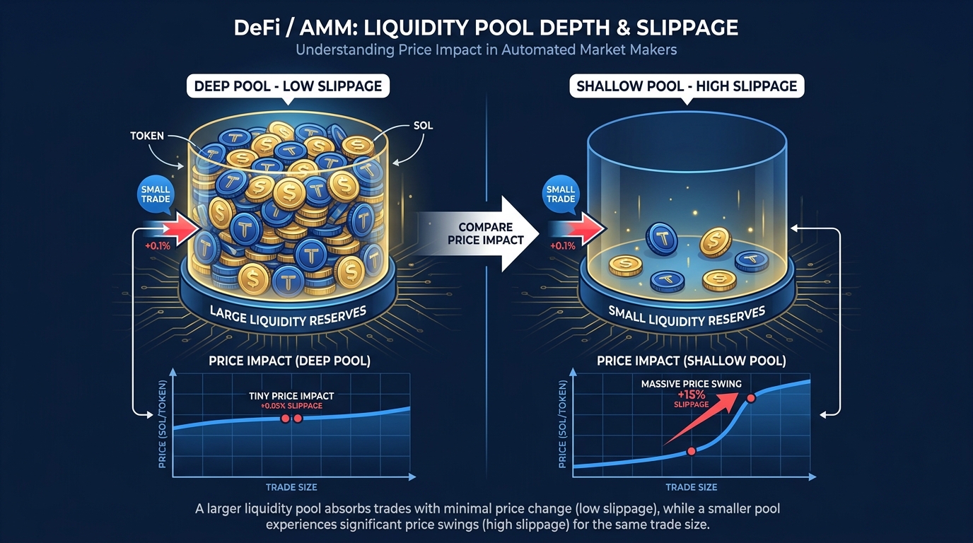
Figure 2:Pool depth matters: A large pool absorbs trades without significant price movement; a thin pool produces wild price swings from even small transactions.
Traditional financial markets solve this with market makers — firms like Citadel Securities or Virtu that continuously post buy and sell quotes, standing ready to transact at any moment. They profit from the spread (the gap between the price they will buy at and the price they will sell at) and from the volume. Their presence provides the liquidity everyone else relies on.
The catch: you cannot just call Citadel and ask them to make a market in your new token. They will not take your call.
This is the promise of decentralized finance — and specifically of the automated market maker.
2Order Books vs. Automated Market Makers
Traditional exchanges operate on order books. You go to a stock exchange and post a limit order: “I will buy 100 shares of Company X at $47.50.” Someone else posts: “I will sell 100 shares at $47.50.” When the prices match, the trade executes. The exchange is just the ledger that records the match.
Order books work well when there are many participants willing to constantly post and update orders. They work poorly for a brand-new token with three holders. You would post your buy order and wait. And wait. Eventually you would either give up or accept a terrible price.
The automated market maker (AMM) solves this by replacing the order book with a pool of assets. Instead of matching buyers with sellers, you match buyers and sellers with a pool of capital that is always available. The pool itself becomes the counterparty for every trade.
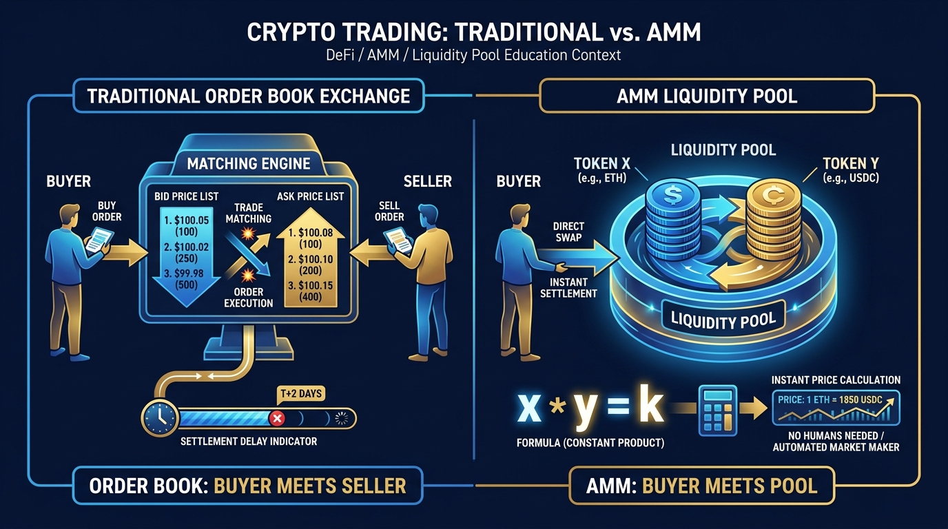
Figure 3:Order book versus AMM: Traditional markets match two humans; AMMs match any human with a pool of capital that is always open.
Think of it like this: an order book is a farmer’s market where buyers and sellers have to physically find each other and agree on a price. An AMM is a vending machine — stocked in advance, priced automatically, open at 3 AM on a Sunday. You do not need another human on the other side. You need capital in the machine.
This analogy holds up remarkably well — except the vending machine reprices itself after every single purchase, and the profit from every transaction goes to whoever stocked the machine in the first place.
3The Constant Product Formula: Two Piles of Coins
The magic behind every AMM — Uniswap, Raydium, Orca, and hundreds of others — is a single mathematical relationship so simple it fits on a napkin:
Here is how to understand it without calculus. Imagine two piles of coins on a table. The left pile contains your token (let us call it LEARN). The right pile contains SOL. The formula says: the product of the two piles must always equal the same number k.
Suppose you start with 1,000 LEARN and 10 SOL on the table. That means k = 10,000. Now a student comes along and wants to buy some LEARN with their SOL. They add 1 SOL to the right pile, bringing it to 11 SOL. To keep the product equal to 10,000, the left pile must shrink: 10,000 ÷ 11 = approximately 909 LEARN. The student received 1,000 - 909 = 91 LEARN for their 1 SOL.
The implied price per LEARN before the trade: 10 SOL ÷ 1,000 LEARN = 0.01 SOL per LEARN. The implied price per LEARN after the trade: 11 SOL ÷ 909 LEARN ≈ 0.0121 SOL per LEARN.
The price went up. Nobody decided that. The math decided it. As more LEARN leaves the pool (because buyers are buying), each remaining token becomes slightly more expensive. As more SOL enters, each token is backed by more SOL. Supply and demand, encoded in arithmetic.
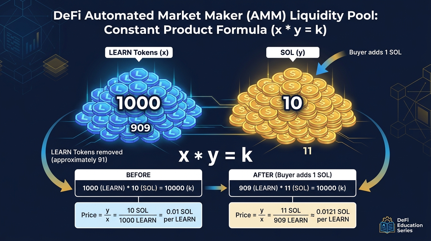
Figure 4:The constant product formula in action: Two piles of coins linked by the rule x·y=k. As one pile grows, the other shrinks, and the ratio between them determines the price.
Where the analogy breaks down: the actual curve in the formula is a hyperbola — the prices do not shift linearly with trade size. Small trades barely move the price. Enormous trades move it dramatically. This non-linear relationship is what creates slippage, discussed shortly.
Where the analogy is revolutionary: this formula runs autonomously on a blockchain, 24 hours a day, for any token pair that has a pool, without any employee, broker, or exchange approval. You seeded that pool. You opened that market.
4Pool Types: Constant Product vs. Concentrated Liquidity
The x·y=k pool has a quiet inefficiency: it spreads your capital across every possible price from zero to infinity. Most of that capital never trades. If LEARN trades between 0.008 and 0.012 SOL all year, the capital positioned to serve trades at 0.0001 SOL or 5 SOL just sits there — committed, earning nothing, waiting for prices that never arrive.
Concentrated liquidity pools fix this by letting each liquidity provider choose a price range. On Solana, the main implementations are Raydium’s CLMM pools, Orca’s Whirlpools, and Meteora’s DLMM. An LP who concentrates the same capital inside a narrow range provides far more depth inside that range — a $1,000 position concentrated in a 20% band can serve trades like a much larger constant-product position would. Traders get better prices; the LP earns a larger share of fees.
The catch is symmetrical: outside your chosen range, your position earns nothing and suffers the full force of impermanent loss. If the price walks out of your band, your capital has been fully converted into the less valuable asset and stops collecting fees until the price walks back. Concentrated liquidity is not passive; it is an active market-making position that needs monitoring and periodic re-ranging.
Think of it as the difference between watering an entire field versus drip-irrigating the rows where crops actually grow. Drip irrigation is dramatically more efficient — as long as you correctly guessed where the crops are.
The rule of thumb for this book: constant product for a new token with no price history (which is exactly what the lab in this chapter uses — you have no idea where your token will trade, so spreading liquidity everywhere is the honest choice); concentrated pools once the price has an established range and there are active LPs willing to manage positions. Pool depth and how to read it are covered further in Chapter 10, Liquidity Depth.
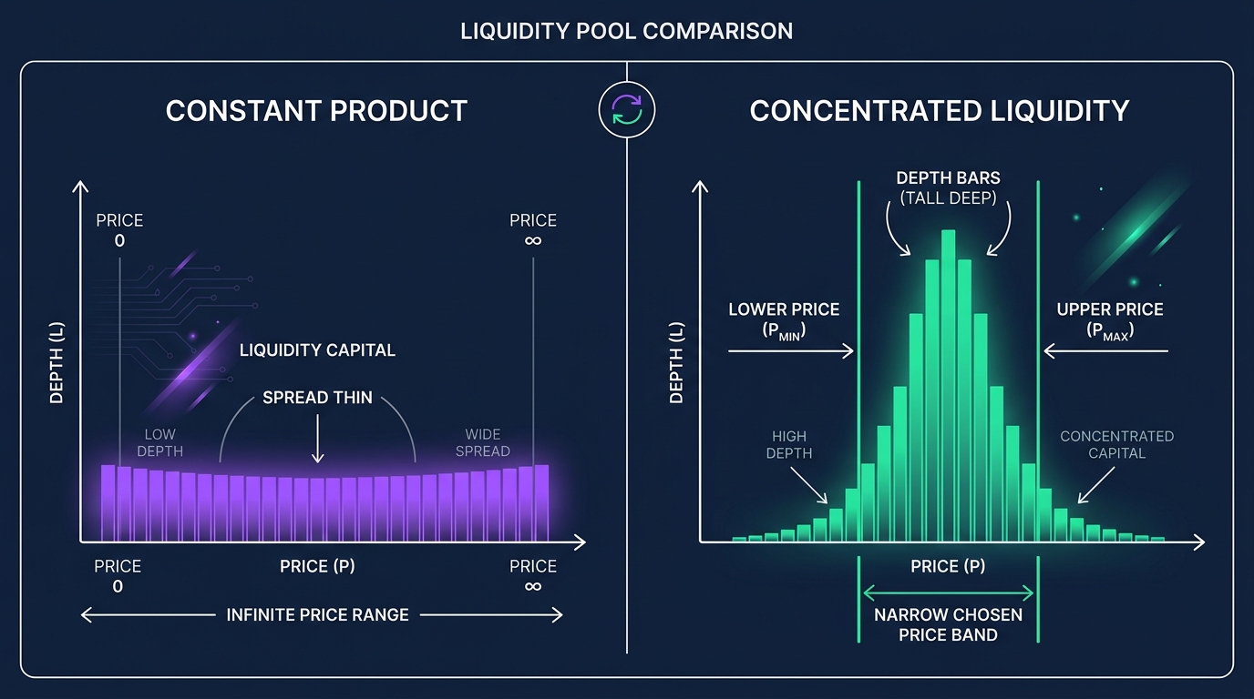
Figure 5:Constant product vs. concentrated liquidity: The same capital spread across all prices (CPMM) versus focused inside a chosen range (CLMM) — more depth in the range, nothing outside it.
5Price Discovery: Why the Pool Wins
In the traditional world, price discovery is a complex negotiation between millions of buyers and sellers, mediated by exchanges and market makers, filtered through bid-ask spreads and clearing delays. In an AMM, price discovery is instantaneous mathematics.
But here is the subtler truth: the pool’s price is not arbitrary. It is anchored to reality by arbitrageurs — traders who profit from price differences between markets.
Suppose the LEARN pool on Raydium shows 0.01 SOL per LEARN, but Jupiter’s aggregated routing finds LEARN trading at 0.012 SOL on a second pool. An arbitrageur instantly buys LEARN from the cheap pool and sells it to the expensive one, pocketing the difference. This trading continues until both pools converge to the same price. The result: all pools stay roughly in sync with each other, and the aggregate price reflects the best available information about what the market values the token at.
You, as the creator, set the opening price by choosing how much SOL to pair with how many tokens when you initialize the pool. But from that moment forward, the market takes over. If you seed 1,000 LEARN against 10 SOL, you have declared the token worth 0.01 SOL each. Whether the market agrees is about to be revealed in real time.
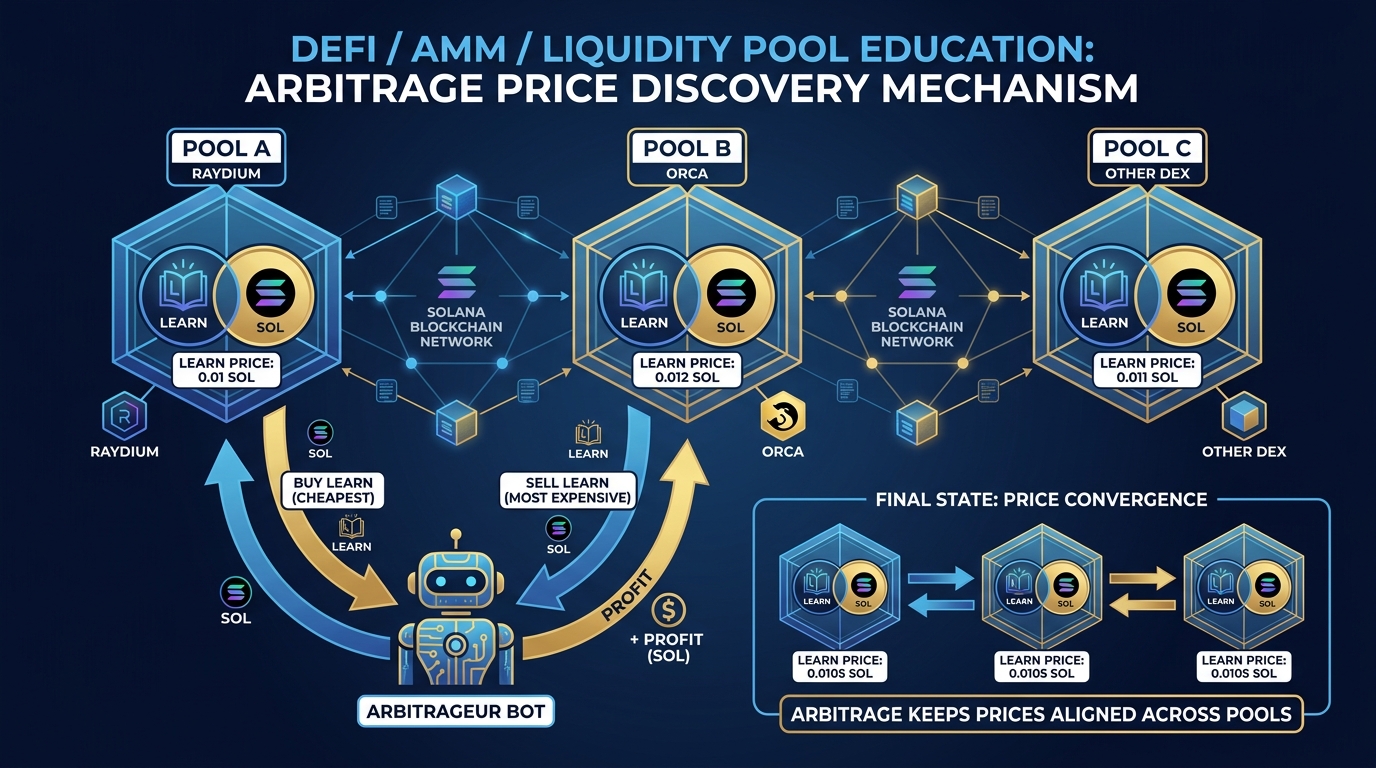
Figure 6:Arbitrage as the invisible hand: When prices diverge across pools, traders immediately profit by bringing them back into alignment — keeping all AMMs in sync without any central coordinator.
6Slippage, Pool Depth, and the Thin Liquidity Problem
Return to the two piles of coins. Suppose instead of 1,000 LEARN and 10 SOL, you started with only 100 LEARN and 1 SOL (the same ratio, k = 100). Now the same student arrives and adds 1 SOL. The pool now has 2 SOL. To maintain k = 100, LEARN drops to 50. The student received 50 LEARN for 1 SOL — a price of 0.02 SOL per LEARN instead of 0.01.
The pool price just doubled because the pool was thin. That is slippage: the difference between the price you expected and the price you actually received.
For practical purposes, this means: if your pool is underfunded, large trades will punish buyers with terrible prices. Sophisticated traders will see the thin pool, flag it as risky, and stay away. Your market will remain illiquid not because nobody wanted to trade but because the economics of trading were too punishing.
The practical lesson: seed your pool with as much capital as you can reasonably afford. For a classroom exercise with $20, you will have a thin pool — and that is exactly the point. You will observe slippage in action when you perform your swap at the end of the activity.
6.1MEV and the Sandwich
Slippage has a predator. Because pending transactions are visible before they execute, a bot can see your swap coming, place a buy immediately before yours, and place a sell immediately after it — pocketing the price impact you created. Your buy pushes the price up; the bot bought cheap just before you and sells into your higher price just after. You are the meat in the sandwich attack, and you pay for both slices of bread.
This is the real reason Jupiter has a slippage-tolerance setting. That setting is the maximum price impact you will accept before your transaction fails — and a high tolerance is an open invitation: it tells a sandwich bot exactly how much it can extract from you before your trade reverts. Sandwiching is one form of MEV (maximal extractable value) — profit extracted by controlling the ordering of transactions. On Solana, MEV largely routes through Jito bundles, and the “MEV tips” paid to validators are part of the staking yield discussed in Chapter 4 (and revisited in Real Yield vs. Emissions Yield later in this chapter).
The practical rule: set slippage as low as the trade will clear, and never use “auto” or unlimited slippage on a thin pool. On a deep pool, a tight tolerance costs you nothing; on a thin pool — like the one you are about to create — it is the difference between a bad price and a much worse one.
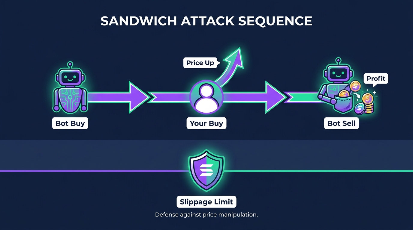
Figure 7:The sandwich attack: A bot front-runs your buy and back-runs it with a sell, capturing the price impact your own trade created. Your slippage tolerance is the ceiling on what it can take.
7LP Tokens and Fees: How Liquidity Providers Earn
When you deposit capital into an AMM pool, you do not simply hand over your tokens. The protocol gives you LP tokens (Liquidity Provider tokens) in return — a claim check that represents your proportional share of the pool.
Think of it like a coat check. You deposit your coat (your LEARN and SOL), you receive a ticket (LP tokens). When you want your coat back, you return the ticket and retrieve your deposit — plus any tips the coat-check staff collected on your behalf during the evening.
The “tips” in this case are trading fees. Every time anyone swaps through your pool, they pay a fee — typically 0.25% of the trade value on Raydium’s Standard AMM pools. That fee is distributed proportionally to all LP token holders. You are not just providing charity; you are running a micro-exchange and earning a cut of every transaction that passes through it.
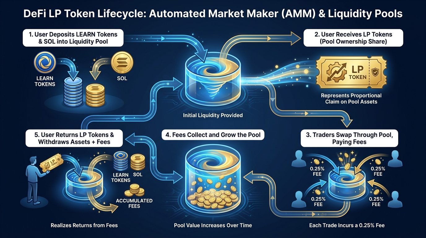
Figure 8:The LP token lifecycle: You deposit two assets, receive a proportional claim (LP token), earn fees from every trade, and eventually withdraw your original capital plus accumulated fees.
There is a trade-off that every liquidity provider must understand: impermanent loss. When you provide liquidity, you hold both assets. If one asset’s price rises dramatically relative to the other, you would have been better off just holding the rising asset. The pool automatically rebalanced against you — selling your winning asset to buy the losing one as the price moved. This loss is “impermanent” because it reverses if the price returns to where it started — but in practice, prices often do not return, and impermanent loss becomes very permanent.
For a classroom token with no external price anchor, impermanent loss is not a major concern. But for real DeFi liquidity provision with established tokens, it is the central risk/reward calculation every LP must make.
Deep Dive: Impermanent Loss Math
Suppose you deposit $100 worth of LEARN and $100 worth of SOL into a pool (50/50 split, standard for most AMMs). If SOL’s price doubles while LEARN stays flat, arbitrageurs will drain your SOL from the pool, replacing it with LEARN, until the ratio reflects the new price. You now have more LEARN and less SOL than you started with — but LEARN did not appreciate. Your pool position is worth less than if you had simply held both assets separately.
The math: if one asset rises by 4x relative to the other, you lose approximately 20% versus a simple hold. The fee income must exceed that loss for LP provision to be profitable — which is why high-volume pools with thin price ratios (like stablecoin pairs) are often the most attractive LP positions.
8Centralized Exchanges as Gatekeepers vs. Decentralized Rails
Here is a question worth sitting with: if you wanted to list your token on Coinbase, what would you do?
You would apply. Coinbase has a listing team. They would review your token for legal compliance, market cap, team background, trading volume, and a dozen other criteria. If they said no — and they almost certainly would for a classroom project — your token would not appear on Coinbase. Ever. Unless circumstances changed and you reapplied.
This gatekeeping is not arbitrary. Coinbase operates under securities regulations, knows-your-customer requirements, and has been sued for listing tokens that later turned out to be unregistered securities. Their caution is rational. But the practical effect is that any token interesting enough to be new and experimental is almost by definition excluded from centralized exchanges.
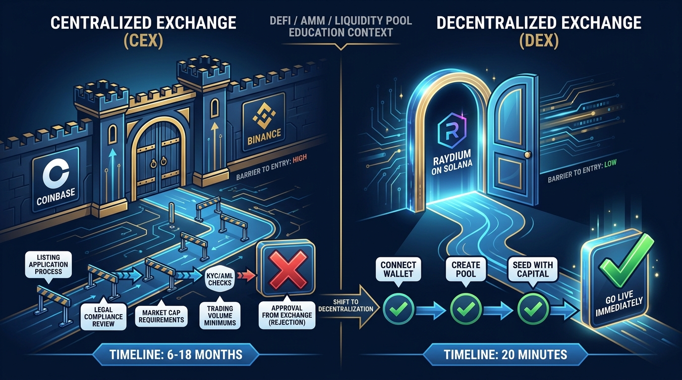
Figure 9:The gatekeeper versus the open rails: A centralized exchange requires approval, legal review, and market maker relationships. A DEX requires only a wallet and a funded pool.
Raydium requires none of this. You connect a wallet with enough SOL to cover transaction fees and pool initialization, create the pool, seed it with capital, and your token is live. Permissionless means literally that — no permission is required from any authority.
Jupiter, Solana’s leading swap aggregator, will automatically find your pool and include it in its routing algorithm. Within minutes of creating your pool, anyone with a Phantom wallet can swap into your token through Jupiter’s interface — exactly the same interface they use to buy SOL, USDC, or any other Solana token. Your classroom project sits next to billion-dollar assets in the same routing engine.
Is this a feature? Is this a danger? We will return to that question at the end of the chapter.
9Launchpads and Bonding Curves
There is a second way to open a market — one that requires no seed capital at all, and one you should understand because it has become the dominant new-token pathway on Solana.
A bonding curve is a pool with only one side. Instead of you depositing tokens and SOL, a program sells tokens along a fixed, pre-programmed price curve: the price starts very low and rises automatically as more tokens are bought. The SOL that buyers pay in stays inside the program. No LP seeding is needed, and the first buyer sets nothing — the curve does. Where your Raydium pool required you to choose an opening ratio and put capital behind it, a bonding curve is the opening price schedule, decided in advance by math.
Launchpads automate this end to end. Anyone creates a token for a few cents; it immediately trades on the curve; and when the curve fills to a threshold — called graduation — the accumulated SOL and remaining tokens are migrated into a regular AMM pool, and the token begins trading like any other. pump.fun is the reference case on Solana: until March 2025, graduated tokens migrated to a Raydium pool; since then they migrate to pump.fun’s own DEX, PumpSwap. Raydium answered with its own launchpad, LaunchLab, whose graduated tokens land in a Raydium CPMM pool — the same pool type you will create in this chapter’s lab.
Why does this matter for a business course? Three reasons. First, sheer volume: launchpads mint thousands of tokens per day and are, by count, how most new Solana tokens are born. Second, they make the “fair launch” argument concrete — no presale, no team allocation, everyone (including the creator) buys on the same public curve. Third, they make rug-pull mechanics visible: the deployer usually buys first, at the very bottom of the curve, which means the deployer’s cost basis is a fraction of every later buyer’s. Watching the deployer’s share on a holders page (which you will do in this lab’s Step 8) is the fastest honest read on a curve token.
Most of what trades on these curves is the memecoin category from Chapter 2 — attention as the underlying asset — and the deployer-buys-first structure is exactly the rug-pull setup Chapter 12 dissects. A bonding curve is neither good nor bad; it is a market-creation machine with the gatekeeping removed even further than Raydium removes it.
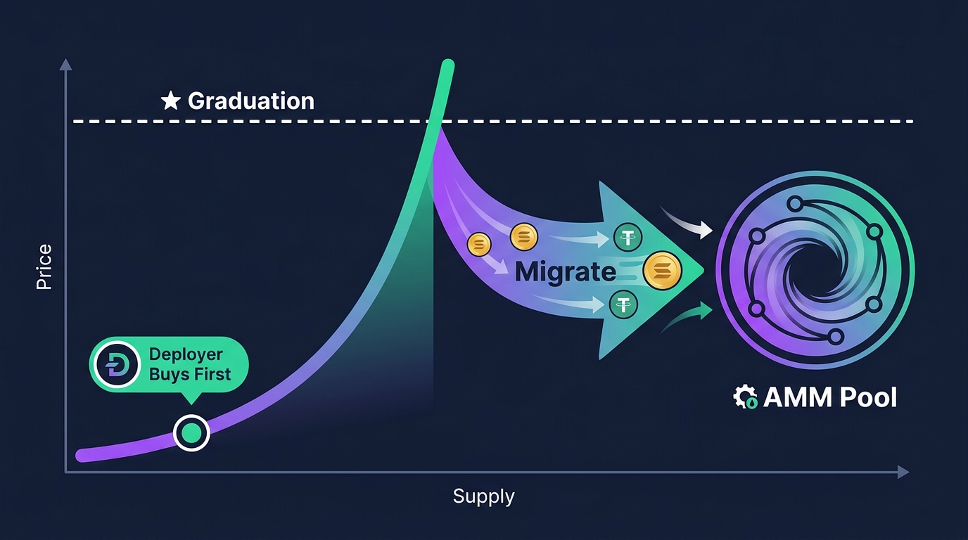
Figure 10:The bonding curve lifecycle: Price climbs along a fixed curve as buyers enter; at the graduation threshold the accumulated SOL and tokens migrate into a standard AMM pool.
10Activity: Open the Market
This is the core lab of Chapter 5. By the end, your token will be live and tradeable, you will hold an LP position, and you will have recorded an actual price-impact observation.
10.1Step 1: Connect to Raydium
Navigate to raydium.io and connect your Phantom wallet using the Connect Wallet button in the top-right corner. Select your wallet and approve the connection. You should see your wallet address and SOL balance displayed.
10.2Step 2: The Liquidity Math — Three Scenarios
Before you touch any interface, do the math. Your opening price is determined entirely by the ratio of tokens to SOL you deposit.
Work through all three scenarios in your notes, then choose one:
Scenario A — 1 SOL, 10,000 tokens
Opening price: 1 SOL ÷ 10,000 LEARN = 0.0001 SOL per LEARN
At SOL = $100, that prices your token at roughly $0.01 each
k = 10,000 (the pool constant for future reference)
Scenario B — 0.5 SOL, 1,000 tokens
Opening price: 0.5 SOL ÷ 1,000 LEARN = 0.0005 SOL per LEARN
At SOL = $100, that prices your token at roughly $0.05 each
k = 500
Scenario C — 0.1 SOL, 100 tokens
Opening price: 0.1 SOL ÷ 100 LEARN = 0.001 SOL per LEARN
At SOL = $100, that prices your token at roughly $0.10 each
k = 10
Record your chosen scenario and the resulting price in your lab notebook.
10.3Step 3: Create the Standard AMM Pool
On Raydium, navigate to Liquidity → Create Pool → Standard AMM. The pool type is labeled Standard AMM (CPMM) in Raydium’s interface — this is the CPMM program, which is what the Pool Types section earlier in this chapter and the Burn & Earn step later in this lab refer to.
You will see two asset selector fields:
Token A: Select SOL
Token B: Paste your token mint address into the search field
Raydium will attempt to look up your token’s metadata. If your token has a proper name and symbol (set in Chapter 3), it will display correctly. If it shows only the raw mint address, that is fine — it will still work.
Enter your chosen amounts from Step 2. The interface will display:
Your initial price (ratio of SOL to your token)
The initial pool reserve amounts
An estimated fee tier
10.4Step 4: Select Your Fee Tier
Raydium offers multiple fee tiers for Standard AMM pools. For a new token with uncertain volume, 0.25% is the standard choice. Higher fee tiers (0.5% or 1%) are more appropriate for very volatile pairs where LPs need compensation for impermanent loss risk.
For a classroom token, stick with 0.25%.
10.5Step 5: Initialize the Pool
Click Initialize Pool. Your Phantom wallet will prompt you to approve two transactions:
A setup transaction (typically small — under 0.01 SOL)
The actual liquidity deposit
Approve both. Raydium charges a one-time 0.15 SOL pool-creation fee (shown in the confirmation), plus under $1 in rent and transaction fees, plus whatever SOL you deposit.
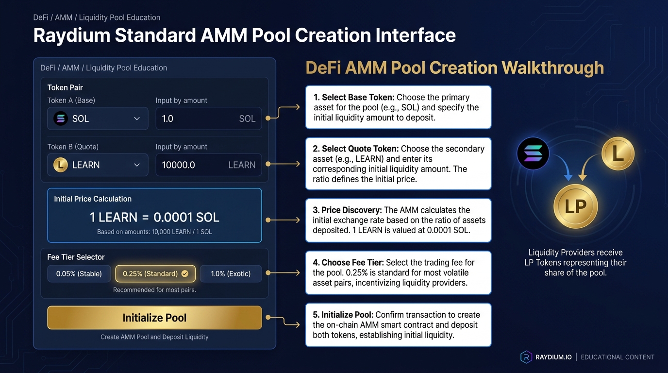
Figure 11:Creating your pool on Raydium: Select your token pair, enter the amounts corresponding to your chosen scenario, confirm the opening price, and initialize.
After the transactions confirm, Raydium will display your LP token balance. Copy the pool address — you will need it for your lab write-up.
10.6Step 6: Perform a Test Swap on Jupiter
Navigate to jup.ag. Connect your Phantom wallet.
In the swap interface:
You Pay: SOL (use a small amount — 0.01 SOL is sufficient)
You Receive: Search for your token by mint address
Jupiter will find your newly created Raydium pool and display a quoted rate. Record the quoted price before executing the swap.
Execute the swap. After it confirms, return to Jupiter and get a new quote for the same trade. Record the new quoted price.
You have just observed slippage and price impact in a live market. The price moved because your pool is small and the trade consumed a meaningful percentage of the pool’s depth.
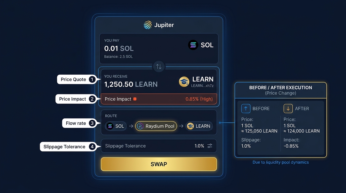
Figure 12:Your token on Jupiter: After pool creation, Jupiter automatically routes trades through your pool. The price shown is derived directly from the constant product formula applied to your pool’s current reserves.
10.7What to Record in Your Lab Notebook
| Item | Value |
|---|---|
| Token mint address | |
| Pool address on Raydium | |
| Scenario chosen (A/B/C) | |
| Opening price (SOL per token) | |
| Opening price (USD per token at current SOL price) | |
| SOL deposited | |
| Tokens deposited | |
| k value (SOL × tokens) | |
| LP token amount received | |
| Quoted price BEFORE test swap | |
| Quoted price AFTER test swap | |
| Price impact percentage | |
| LP locked/burned (Y/N, %) | |
| RugCheck score | |
| Slippage tolerance used on the Jupiter swap |
10.8Verify Your Pool on Solscan
Navigate to solscan.io and search for your pool address. You should see the pool’s transaction history, current reserves, and the liquidity add event from your initialization. This is your pool’s permanent, public, immutable record.
10.9Step 7: Lock It (10 min)
The “Standard AMM” pool you created is a Raydium CPMM pool, and Raydium’s Burn & Earn can lock it permanently while you keep the right to collect its trading fees. On Raydium go to Liquidity → Create → Burn & Earn, select your position, read the confirmation (it shows the position address, size, and pool), type the confirmation sentence the screen asks for, and click Confirm. The lock is irreversible; a Fee Key NFT arrives in your wallet — whoever holds it can claim the locked position’s fees. If you want to keep your capital for later chapters, do not lock; instead read the Burn & Earn screen up to the confirmation, close it, and complete step 2 by observation.
Open rugcheck.xyz, paste your mint address. Record the risk score and each line item: mint authority, freeze authority, LP locked %, top holders. Take a screenshot before and (if you locked) after.
Write two sentences: what a buyer sees on RugCheck for your token today, and what one change would most improve it.
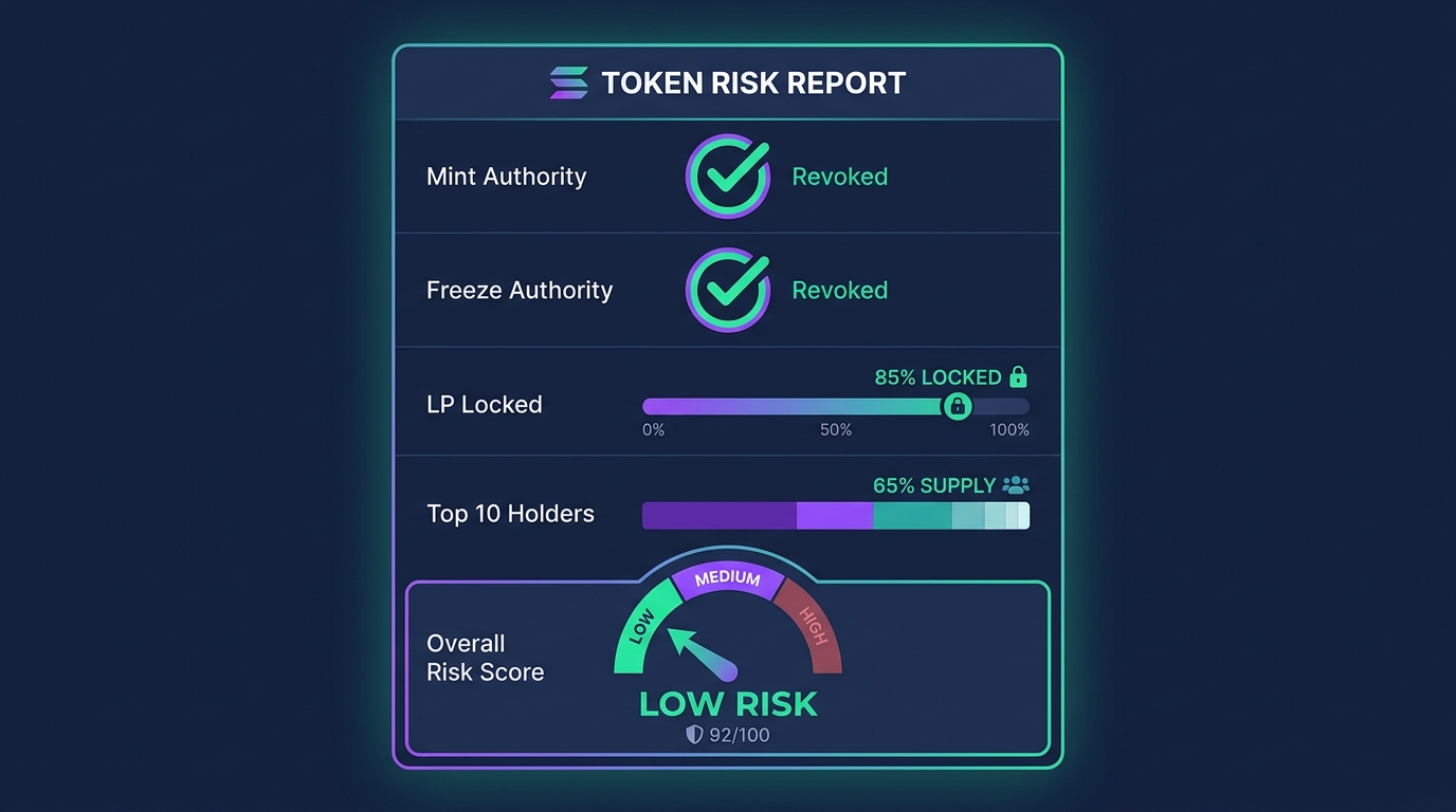
Figure 13:Reading a RugCheck report: Risk score, mint and freeze authority status, LP locked percentage, and holder concentration — the one-glance summary a buyer runs on your token before touching it.
10.10Step 8: Watch a Bonding Curve (10 min, observation only, no purchase)
Open pump.fun. Pick any token on the board. Note the bonding curve progress percentage and the market cap.
Find the same token on DexScreener by pasting its address. If it has migrated, note the pool it migrated to and the moment of migration in the chart.
Open its Solscan holders tab. Record the deployer’s share (usually the top non-pool wallet).
Write two sentences: what happens to the price the moment the curve migrates, and what would you check before buying anything on a curve?
11🔬 Hands-On Lab: DeFi in an Afternoon (90 min, mainnet, ≈ $10 at risk)
This lab is designed for a second class session. Every step uses small amounts; every step ends with something recorded.
11.1Part A — Hold a Dollar (10 min)
In Phantom, click Swap. From: SOL. To: USDC. Amount: 0.02 SOL. Record the quoted rate, the route Phantom shows (which pools it used), and the fee. Confirm.
On Solscan, search the USDC mint
EPjFWdd5AufqSSqeM2qN1xzybapC8G4wEGGkZwyTDt1v. Record Mint Authority and Freeze Authority. Note the freeze authority is not “None.”Open the Holders tab. Record holder count and the largest holder.
Write two sentences: what can the issuer do to your USDC that no one can do to your SOL, and why might a business hold USDC anyway?
11.2Part B — Stake It (15 min)
Native staking, by observation (Phantom requires a minimum of 1 SOL to stake natively, so most students will not execute this): in Phantom’s token list open Solana → More → Stake SOL → Native Staking. Phantom shows a validator list with each validator’s commission and estimated APY. Record the commission and APY of the top suggestion, then look the same validator up on solanacompass.com (or validators.app) and record its uptime/skip rate. Close without staking. (A student with ≥1 SOL to spare may stake it: click Stake, then record the stake account address; unstaking is under Native Stakes → Other → Unstake and takes until the next epoch.)
Liquid staking, executed: open marinade.finance, click Stake, connect Phantom, and stake 0.05 SOL. Record the SOL→mSOL exchange rate you received (mSOL received ÷ SOL deposited), the displayed APY, and the transaction signature. Confirm mSOL appears in Phantom.
Open jito.network. Record JitoSOL’s displayed APY and the line showing MEV rewards. Do not transact.
Find Solana’s current inflation rate (Solscan’s or the explorer’s supply page shows it). Write three sentences: how much of each of the three yields is emissions vs. real fees/MEV, and which one is Chapter 4’s “circular yield”?
11.3Part C — Borrow Against It (25 min)
Open app.kamino.finance and connect Phantom. Open Borrow/Lend and select the Main Market. Each asset row shows its supply APY, borrow APY, and maximum loan-to-value. (app.marginfi.com is an equivalent alternative with a Lend page and the same fields.)
Click SOL → Supply and deposit 0.05 SOL (or the mSOL from Part B — a staked asset can also be collateral). Record the supply APY.
Click USDC → Borrow and borrow 1 USDC (the app enforces a minimum; take the smallest it allows). Your position panel now shows Net Value, LTV, Liquidation LTV, and a Health gauge. Record all four.
Record the SOL price at which the app says your position would be liquidated. Check it: liquidation occurs when debt ÷ collateral value reaches the Liquidation LTV.
Repay the USDC and withdraw the collateral. Record total interest paid.
Search the market list for your Chapter 3 token. It is not there. Write two sentences: which two things from this chapter and Chapter 10 would a lending market require before listing it?
11.4Part D — Find the Oracle (10 min)
Open pyth
.network /price -feeds /crypto -sol -usd. Record the price, the confidence interval, and the number of publishers. Compare to the SOL price shown in your own Raydium pool from earlier in this chapter (SOL per LEARN inverted). Write one sentence: why must the lending market in Part C read Pyth rather than a pool?
11.5Part E — Read the Map (10 min)
Open defillama
.com /chain /Solana. Record total TVL and the top five protocols. Label each as DEX, lending, liquid staking, or other. Find the protocol you used in Part C and the one you used in Part B. Record their TVL.
Write three sentences: which lego did your money touch in which order today, where would a bug in any one of them have left you, and which single risk from DeFi Risk worried you most while doing it?
11.6Deliverable — The DeFi Lab Sheet
A one-page table with every recorded value from Parts A–E, the five short written answers, and the transaction signatures for the swap, the stake, the deposit, the borrow, and the repayment.
12Reading Your Position Over Time
Your LP position has a live value. If you return to Raydium’s liquidity dashboard, you will see your pool listed under My Positions. It will show:
Current total value of the pool
Your percentage ownership (since you own 100% — you are the only LP)
Accumulated fees (likely $0.00 for now, until others trade through your pool)
Any impermanent loss (will be minimal for a classroom token with low external price movement)
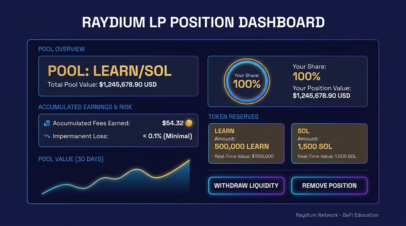
Figure 14:Your LP dashboard on Raydium: Track your pool’s value, ownership stake, fee earnings, and impermanent loss in real time — all from on-chain state, no trusted third party required.
13Managing Liquidity After Launch
Opening the pool is day one. What you do with it afterward is a signal every buyer reads.
Adding liquidity as demand grows. As trading volume and holder count rise, a thin pool becomes the bottleneck: every meaningful trade moves the price, and serious buyers stay away. Adding liquidity — more of your token paired with more SOL or USDC — deepens the pool and shrinks slippage. Treasuries typically add in scheduled increments as volume justifies it, rather than all at once.
Removing liquidity — and why a buyer reads it as a warning. You can withdraw your LP position at any time; it is your capital. But every on-chain observer can see the removal, and the default interpretation is the worst one: the creator is heading for the exit. A rug pull is a liquidity removal — the creator drains the pool’s SOL and leaves holders with a token that cannot be sold. Even a legitimate partial withdrawal (say, to fund operations) will be read through that lens. If you must remove liquidity, announce it first, explain it, and do it on a schedule.
Protocol-owned liquidity. The stronger pattern is for the project’s treasury — not the founder’s personal wallet — to hold the LP position. The treasury earns the trading fees, the liquidity cannot vanish on one person’s decision, and (once governance exists) removal requires a vote. Chapter 11 covers treasury custody through multisigs and DAOs; protocol-owned liquidity is one of the healthiest assets a treasury can hold.
Locking or burning LP tokens. The most credible commitment a creator can make is to give up the ability to drain the pool at all: send the LP tokens to a locking contract (or burn them outright), so the pooled capital can never be withdrawn. Raydium’s Burn & Earn — which you will use or observe in Step 7 of this chapter’s lab — locks the position permanently while still letting the holder of a Fee Key NFT collect trading fees. On-chain, “LP locked” is the single line item that most distinguishes a project from a rug-pull setup (Chapter 12 covers the mechanics of the scam itself).
Market makers and CEX listings. Eventually a successful token outgrows a single AMM pool: a professional market maker can quote it on multiple venues, and a centralized exchange listing brings custodial users who will never touch a DEX. Both belong late in the sequence — only after organic volume and holder count justify them (the Chapter 10 metrics tell you when). Paying a market maker or chasing a listing before there is organic demand buys the appearance of a market, not a market.
14Beyond the Pool: The DeFi Stack
The pool you just built is one of five primitives that, composed together, are what “decentralized finance” actually means: a stable unit of account, a yield on the base asset, a way to borrow against what you hold, a source of truth for prices, and markets to trade all of it. You have the last one. This section walks through the other four.
Each primitive is a program (Chapter 8) that anyone can call, and each can call the others — the industry’s phrase is “money legos.” A lending market calls the token program to move collateral; an aggregator calls a dozen pools to route one swap; a liquid-staking token minted by one program becomes collateral inside another. The composition is the point, and it is also the risk, which is why this section ends with DeFi Risk. Everything here is done by observation or with a few dollars in the lab that follows.
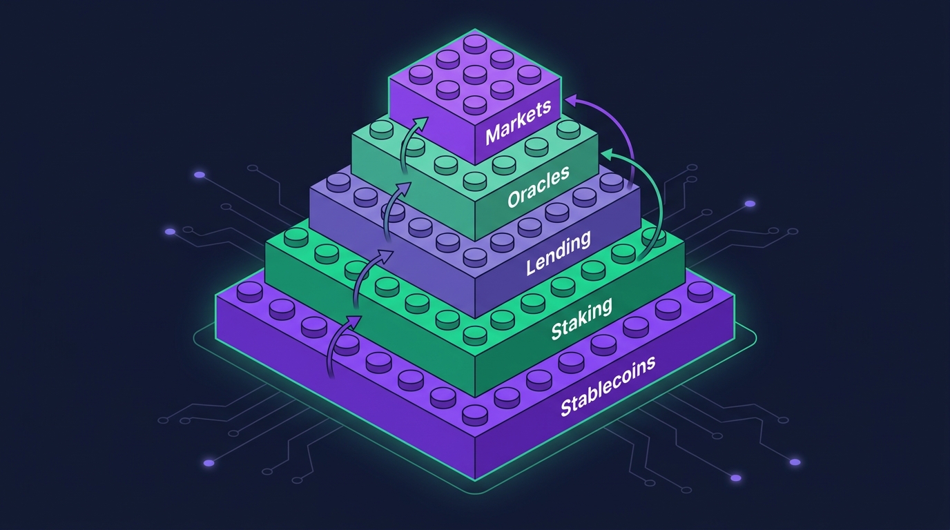
Figure 15:The five money legos: Stablecoins (the unit of account), staking (yield on the base asset), lending (borrowing against holdings), oracles (the price feed), and pools (the markets) — each a program, each composable with the others.
14.11. Stablecoins: The Unit of Account
A stablecoin is a token designed to hold a fixed value against a reference asset — almost always the U.S. dollar. USDC is issued natively on Solana and is the quiet workhorse of everything this book has described: it is the quote asset for most serious pools, the treasury asset Chapter 4 recommends holding, and the “convert immediately” target for merchants in Chapter 7. When DeFi needs a dollar, it uses a stablecoin.
Not all stablecoins are stable for the same reason. There are three backing models, and the differences matter enormously:
Fiat-reserve — USDC. The issuer holds actual cash and short-term U.S. Treasuries equal to the tokens outstanding and publishes attestations. The token is a claim on a regulated reserve.
Crypto-collateralized — DAI. Over-collateralized by other crypto assets locked in smart contracts, with the parameters (which collateral, what ratios) set by MakerDAO governance (the DAO structure Chapter 11 covers). No bank account required — but the collateral itself is volatile, hence the over-collateralization.
Algorithmic — Terra/UST, May 2022. No reserve at all; the peg was maintained by an arbitrage loop with a sister token. When confidence broke, the loop ran in reverse and roughly $40 billion evaporated in days. It is the cautionary case, and the reason “how is it backed?” is the first question to ask of any stablecoin.
There is a custody twist that ties back to Chapter 1. USDC’s mint keeps a freeze authority held by the issuer — the same authority you examined on your own token in Chapter 3 — and the issuer can freeze any USDC account. It has done so, under sanctions orders. “Not your keys, not your coins” has a corollary: “not your issuer, not your dollars.” Self-custodying USDC protects you from exchange failure, but not from the issuer itself.
Nor is the peg a law of nature. In March 2023, USDC traded near $0.88 for a weekend when part of its reserves sat in a bank that had just failed. The peg recovered when the U.S. government backstopped the bank’s deposits — but the lesson stands: a stablecoin is exactly as stable as its reserves and its redemption path. Depeg is the word for the failure mode.
Regulation has now caught up. The GENIUS Act, signed into U.S. law in July 2025, is the first federal stablecoin framework: it limits issuance to licensed “permitted payment stablecoin issuers,” requires 1:1 reserves in cash and short-term Treasuries, mandates monthly reserve disclosures, and guarantees redemption at par. Implementing regulations were issued by the OCC and Treasury through 2026, with the framework taking full effect in early 2027. Chapter 12’s regulatory snapshot places this in the broader legal landscape.
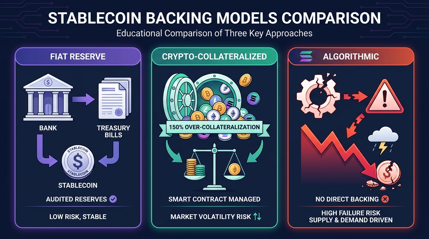
Figure 16:Three backing models: Fiat reserves (USDC), crypto over-collateralization (DAI), and the algorithmic loop (UST — the one that collapsed). A stablecoin is as stable as whatever stands behind it.
14.22. Staking and Liquid Staking: Yield on the Base Asset
Native staking is Solana’s built-in yield. You delegate SOL to a validator; the validator votes on blocks; and the network’s inflation rewards (the 8% declining toward 1.5% schedule from Chapter 4) flow to stakers, minus the validator’s commission. Two properties matter. First, delegation is not custody — the SOL never leaves your control; the validator can vote with your stake’s weight but cannot spend it. Second, unstaking is not instant: it takes effect at the end of an epoch, roughly two to three days.
Liquid staking removes the lockup by adding a layer. You deposit SOL into a protocol like Marinade or Jito and receive a liquid staking token — mSOL or JitoSOL — that represents your staked position. The token rises in value against SOL as rewards accrue, and because it is just an SPL token, it can be traded, pooled, or posted as loan collateral while still earning staking yield. Your capital works twice.
What liquid staking adds, it also charges for: smart-contract risk (the staking protocol is a program that can have bugs) and a second market — the LST trades on its own pools and can trade at a discount to the SOL it represents if too many holders want out at once and the unstaking queue backs up.
One sentence on restaking — using staked assets to secure additional protocols for additional yield — which exists on Solana but layers risk on risk and is beyond this book’s scope.
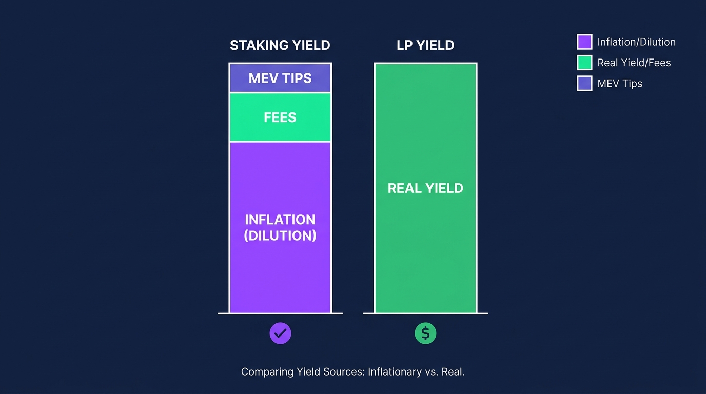
Figure 17:Where staking yield comes from: Mostly inflation (dilution redistributed to stakers), plus smaller shares of real transaction fees and MEV tips. Liquid staking tokens pass the same yield through a program layer.
14.33. Lending Markets: Borrowing Against What You Hold
A lending market is the second kind of pool. Where your AMM pool holds two assets and prices trades between them, a lending pool holds one asset supplied by depositors who earn interest, and lends it to borrowers who post different assets as collateral. The interest rate is not set by anyone: it follows a utilization curve — the greater the share of the pool that is currently borrowed, the higher the rate, so lending markets self-balance the way your AMM self-prices. On Solana, Kamino and Marginfi are two established lending markets (the lab uses one of them).
The core safety mechanism is over-collateralization. Post $100 of SOL and you can borrow up to roughly $70 of USDC at a 70% loan-to-value ratio. Your position’s health factor = collateral value × liquidation threshold ÷ debt. As long as it stays above 1.0, you are safe. The moment it drops below 1.0 — because your collateral fell in price or your debt grew — anyone may liquidate you: repay your debt and take your collateral at a discount. Liquidation is not a penalty imposed by a loan officer; it is an open bounty, claimed by bots within the same block.
Why does this matter for your token? Two reasons, one attractive and one dangerous. The attractive one: “collateral” is the deepest utility sink in Chapter 4’s list — tokens posted as collateral are locked, out of circulation, for as long as the loan lasts. A token that lending markets accept as collateral has structural demand. The dangerous one: a thin pool (the thin liquidity problem from earlier in this chapter) means one large sale drops the price, which drops every borrower’s health factor, which triggers liquidations, which sell more collateral into the same thin pool, which drops the price further — the liquidation cascade. This is why lending markets list only tokens with deep liquidity and a reliable price feed. Which raises the question: reliable according to whom? That is the next primitive.
Where the analogy breaks down: a bank calls you before foreclosing; a lending program liquidates in the very block your health factor crosses 1.0. There is no phone call, no grace period, no negotiation. The rulebook is the loan officer.
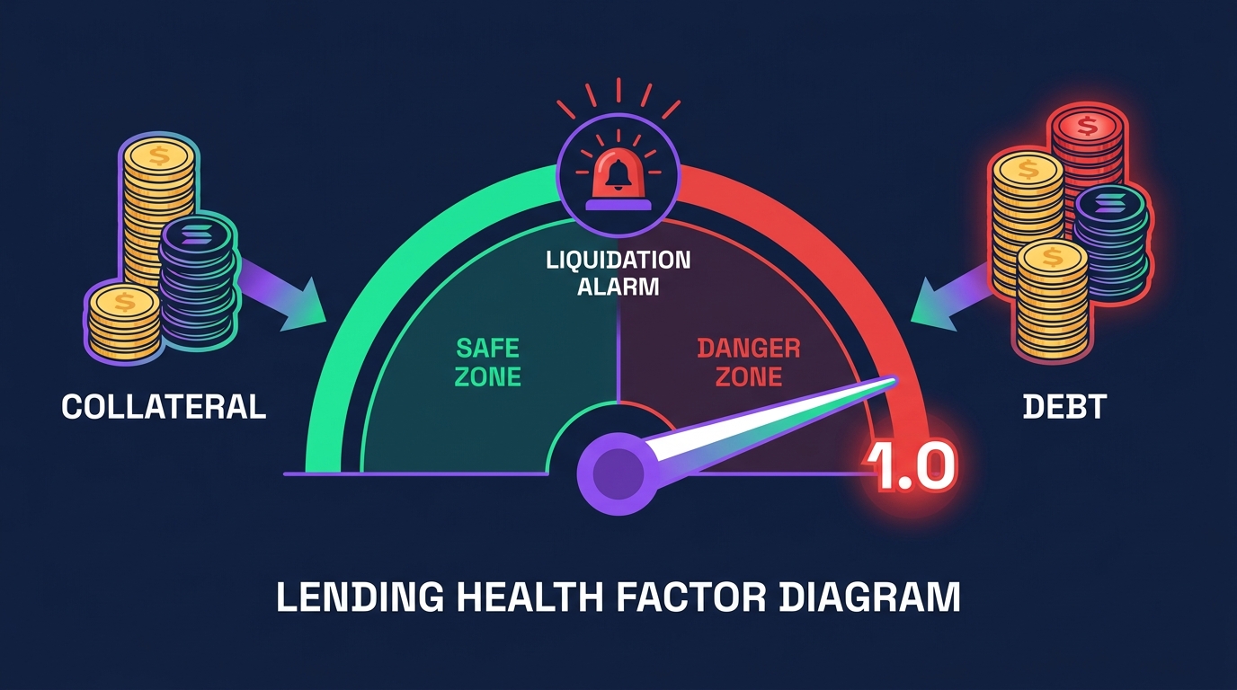
Figure 18:The health factor: Collateral value × liquidation threshold ÷ debt. Above 1.0 you are safe; the block it crosses below, anyone may repay your debt and claim your collateral at a discount.
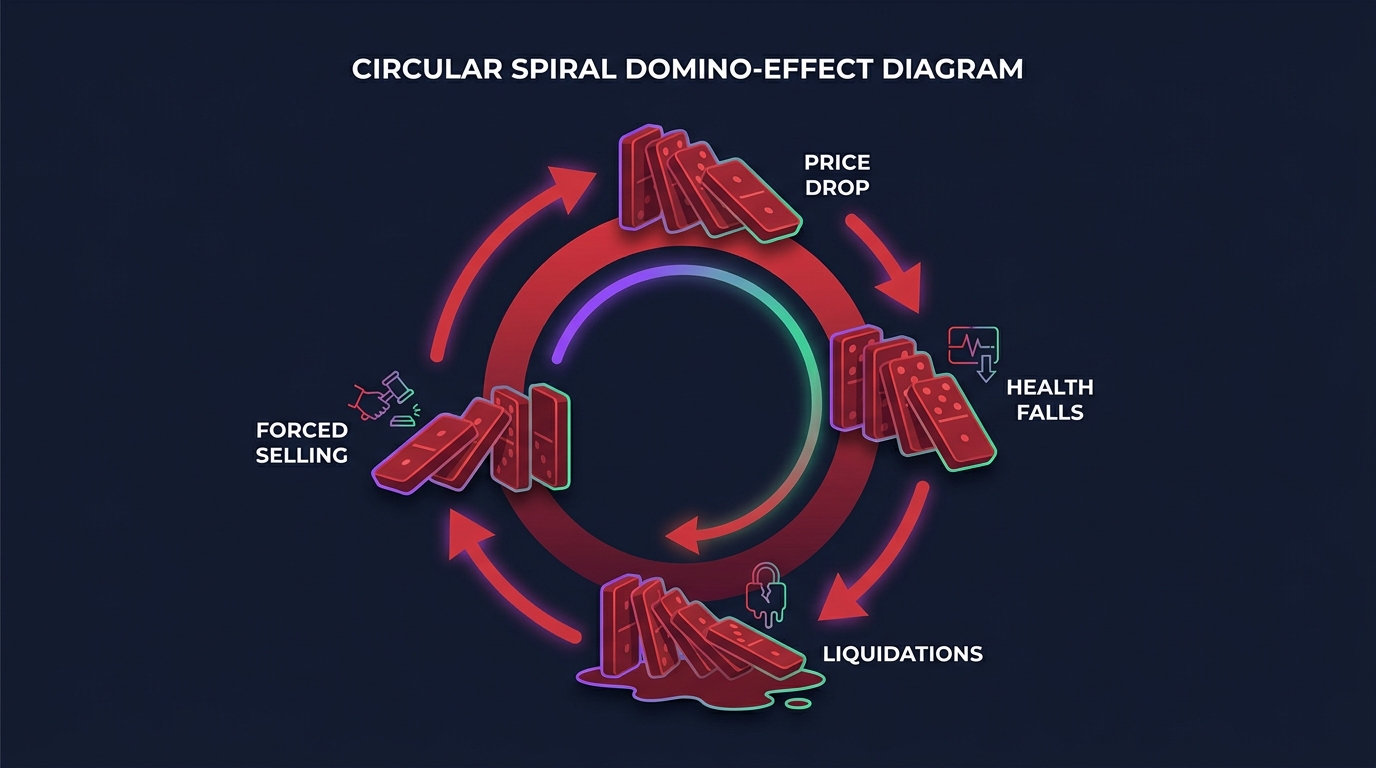
Figure 19:The cascade: Price drop → health factors fall → liquidations fire → collateral is sold into a thin pool → price drops further. Thin liquidity turns one sale into a chain reaction.
14.44. Oracles: Where the Price Comes From
A lending market cannot read prices from one pool, because a pool can be pushed — you saw in the slippage section how a single trade moves a thin pool’s price. If Kamino valued your collateral off one pool, an attacker could shove that pool’s price up, borrow against the inflated value, and walk away.
Instead, it reads a price oracle: an on-chain price feed aggregated from many venues. On Solana, the leading oracle is Pyth — a network of dozens of publishers (exchanges, market makers, trading firms) each contributing prices, aggregated into a single feed that carries both a price and a confidence interval (how much the publishers disagree). Switchboard is the other established Solana oracle.
Everything downstream depends on the oracle: every liquidation in every lending market, every dollar-denominated token price (Chapter 7’s Pricing Problem), every real-world-asset token (Chapter 2). And because everything depends on it, it is a prime target — oracle manipulation and stale feeds sit behind a large share of DeFi exploits, which is why it appears again in DeFi Risk below.
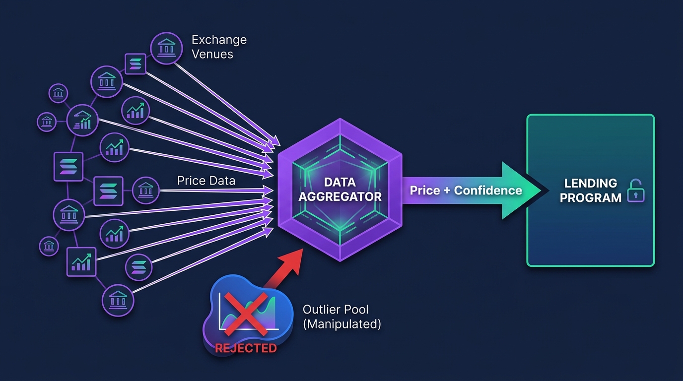
Figure 20:The oracle flow: Many publishers → one aggregated feed with a confidence interval → every lending market, pricing engine, and RWA token downstream. One pool can be pushed; dozens of publishers are much harder.
14.55. Real Yield vs. Emissions Yield
Here is the test that ties this section back to Chapter 4’s “Circular Yield” failure pattern, and it fits in one sentence: what asset is the yield paid in, and where did that asset come from?
Apply it to what you have seen. SOL staking yield is mostly inflation — new SOL minted by the schedule from Chapter 4, which is dilution redistributed to stakers — plus a smaller share of real transaction fees and MEV tips (see MEV and the Sandwich earlier in this chapter). LP fees from your pool are real yield: paid by actual traders, in assets they gave up, for a service you provided. A protocol advertising “40% APY paid in its own token” is emissions yield — the protocol is printing its own token and handing it to you — unless a genuine fee stream backs the number.
A three-line worked example with your LEARN pool:
Real yield: your pool earns 0.25% of every trade. If $40 of volume flows through your $20 pool in a month, you earned $0.10 in fees — $0.10 ÷ $20 = 0.5% monthly, ≈ 6% annualized, paid in SOL and LEARN that traders actually spent.
Emissions yield: now suppose you also “reward” yourself by minting 100 new LEARN per month to LPs and advertise the combined figure as “45% APY.” The extra 39 points were printed, not earned; every LEARN holder paid for them through dilution.
The test: delete the emissions line and see what remains. What remains (6%, from fees) is the business. The rest is Chapter 4’s circular yield with better marketing.
14.66. DeFi Risk
Composability is why DeFi is powerful and why it fails in chains. Five named risks, and what each looks like:
Smart-contract risk. Every primitive above is a program, and programs have bugs. An exploit in a lending market or staking protocol can drain everything it holds, instantly and irreversibly. Chapter 8’s auditor checklist covers what auditors look for; the practical takeaway is that “audited” is a minimum bar, not a guarantee.
Oracle manipulation. Push a thin pool’s price so a lending market mis-values collateral — borrow real assets against fake value and vanish. This is why serious protocols read Pyth rather than pools, and why a confidence interval exists: when publishers disagree sharply, downstream protocols can pause rather than trust a suspect price.
Liquidation cascades. Covered above: falling prices trigger liquidations that force sales that drop prices further. Cascades turn a bad day into a wipeout precisely in the thin-liquidity conditions this chapter taught you to recognize.
Bridge risk. Assets wrapped from another chain depend entirely on the bridge’s security — the locked originals on chain A are the only thing backing the wrapped copies on chain B. Bridges concentrate enormous pooled value behind one attack surface, and they account for the industry’s largest single losses (the Chapter 0 box names Wormhole and Ronin). A wrapped asset is only as good as its bridge.
Composability risk. The failure that arrives from a direction you do not control: a protocol you integrated is exploited, and suddenly your token is the collateral being dumped, or the pool you route through is drained, or the LST you accepted is depegging. When you compose with another protocol, you inherit its attack surface.
The defenses, for a builder or a buyer: integrate only audited protocols; prefer oracle-based pricing over pool-based; watch whether your token is listed as collateral anywhere (Chapter 10’s monitoring); and never post more than you can afford to lose to liquidation.
14.77. The DeFi Map
The industry’s headline metric is total value locked (TVL) — the dollar value of all assets deposited in a protocol’s contracts — and the place to read it is DeFiLlama, which breaks TVL down by chain and by protocol. Ten minutes on DeFiLlama’s Solana page teaches you the shape of the whole landscape: the top protocols sort visibly into the categories this section just walked through — DEXes (pools like yours), lending markets, liquid staking, and perpetuals exchanges. One caveat before you quote a TVL number: it counts the same dollar more than once when assets are re-deposited across legos — the SOL you liquid-stake into mSOL and then deposit as lending collateral appears in both protocols’ TVL. The map is honest; the total is generous.
15The Broader Picture: What You Just Built
Take a moment to understand what just happened. You created a functioning financial market from scratch, on a global network, in about 20 minutes, for less than $20 in capital plus a few cents in transaction fees.
The pool you created will:
Accept trades 24 hours a day, 365 days a year
Price those trades algorithmically, without your involvement
Distribute fees to you as the LP
Remain accessible to any wallet in the world
In 2000, building a trading market for a new financial instrument required a broker-dealer license, a registered exchange, clearing relationships, market-maker agreements, compliance staff, and millions of dollars in capital. The shortest path was years, not hours.
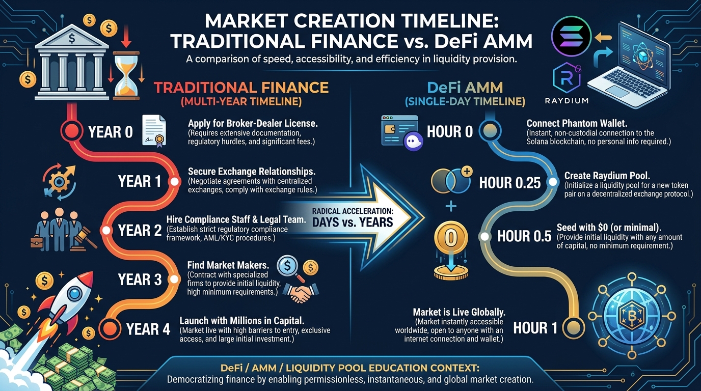
Figure 21:Compressed market creation: What required regulatory approvals, exchange listings, and market-maker agreements for legacy finance now takes a wallet, a small capital allocation, and a few on-chain transactions.
Is this revolutionary? Undeniably. Is it dangerous? That depends entirely on who you ask — and perhaps on which side of the trade you are on.
16🎯 In-Class Assignment: Open Your Market (10 pts)
Details and instructions will be provided in class.
Points: 10
17Discussion: Feature or Danger?
The same guidelines below apply to this prompt.
17.1Discussion Guidelines
Write a substantive response (minimum 250 words) that takes a clear position on the feature-versus-danger question. Your response should:
Distinguish between the perspective of the creator (who controls the initial liquidity and token supply) and the perspective of the buyer (who has no insight into the creator’s intentions)
Include at least one scholarly or credible citation — this could be an academic paper on DeFi market manipulation, a regulatory filing, a journalistic investigation of a rug pull, or a legal analysis of AMM governance
Avoid purely descriptive answers — argue for a position, acknowledge the strongest counterargument, then defend your view
After posting your initial response, reply to at least two classmates with substantive engagement — not just “I agree.” Push back on assumptions, introduce evidence they may have missed, or extend their argument into a domain they did not consider.
Do not describe small-group debate formats or in-class discussion structures — this is an individual written assignment.
18Glossary
Liquidity The ease with which an asset can be bought or sold at a stable price. High liquidity means large trades can occur without significant price movement; low liquidity means even small trades can cause dramatic price swings.
Automated Market Maker (AMM) A type of decentralized exchange protocol that uses mathematical formulas — rather than order books — to price assets and execute trades. The pool of capital is the counterparty for every transaction.
Constant Product Formula The mathematical rule x·y=k that governs most AMMs. The product of the two token reserves in a pool must remain constant, which means that as one reserve decreases, the other increases proportionally, causing the price ratio between them to shift.
Pool Depth The total value of assets locked in a liquidity pool. Deeper pools produce less slippage for a given trade size; shallower pools produce more.
Slippage The difference between the expected price of a trade and the actual executed price. In AMMs, slippage increases with trade size relative to pool depth.
LP Token A token issued to a liquidity provider representing their proportional share of a pool. LP tokens can be redeemed to withdraw the underlying assets plus any accumulated fees.
Impermanent Loss The opportunity cost experienced by liquidity providers when the price ratio between the two pooled assets changes from the ratio at the time of deposit. The loss is “impermanent” only if prices return to their original ratio.
Price Impact The effect of a trade on the quoted market price within a pool. Large trades in small pools produce high price impact; small trades in large pools produce negligible impact.
Fee Tier The percentage of each trade’s value charged as a fee and distributed to liquidity providers. Common tiers are 0.01%, 0.05%, 0.25%, and 1%.
Price Discovery The process by which a market determines the fair value of an asset through the interaction of supply and demand. In AMMs, price discovery is maintained through arbitrage trading that links pools across platforms.
Arbitrageur A trader who profits from price differences between markets, simultaneously buying from the cheaper source and selling to the more expensive one. Arbitrageurs keep AMM prices aligned with each other and with external markets.
Raydium A major Solana DEX offering constant-product (Standard/CPMM) and concentrated-liquidity (CLMM) pools, integrated with the Jupiter aggregator.
Jupiter Solana’s leading swap aggregator, which finds the best available price across all DEX pools on the network and routes trades accordingly. Any pool created on Raydium is automatically accessible through Jupiter.
Permissionless Describing a system that any participant can access without approval from a gatekeeper. AMM pool creation is permissionless — no exchange approval, no license, no regulatory filing is required.
Standard AMM Raydium’s basic pool type, which implements the constant product formula. Suitable for most token pairs, including newly launched tokens with limited price history.
Concentrated Liquidity A pool design (Raydium CLMM, Orca Whirlpools, Meteora DLMM) in which each liquidity provider chooses a price range for their capital, providing far more depth inside the range than a constant-product position of the same size — and earning nothing, while suffering full impermanent loss, outside it.
MEV Maximal extractable value: profit extracted by controlling the ordering of transactions — for example, placing trades immediately before and after a visible pending swap. On Solana, MEV largely routes through Jito bundles, and MEV tips form part of staking yield.
Sandwich Attack A form of MEV in which a bot places a buy immediately before a victim’s swap and a sell immediately after it, pocketing the price impact the victim’s trade created. A high slippage tolerance is the attacker’s budget.
Bonding Curve A one-sided pool in which a program sells tokens along a fixed price curve — price rises as more are bought — and holds the SOL it receives. No liquidity seeding is required; the curve itself is the opening price schedule.
Launchpad A platform (pump.fun, Raydium LaunchLab) that automates token creation and bonding-curve trading; when the curve fills to a threshold (“graduation”), the accumulated SOL and tokens migrate into an AMM pool.
Protocol-Owned Liquidity An LP position held by a project’s treasury rather than a founder’s personal wallet, so trading fees accrue to the treasury and the liquidity cannot be withdrawn on one person’s decision.
Liquidity Lock Sending LP tokens to a locking contract (or burning them) so the pooled capital can never be withdrawn — the credible on-chain commitment that a pool cannot be drained. Raydium’s Burn & Earn locks a position permanently while a Fee Key NFT retains the right to collect its fees.
Stablecoin A token designed to hold a fixed value against a reference asset, almost always the U.S. dollar. USDC is the dominant stablecoin issued natively on Solana.
Fiat-Reserve Stablecoin A stablecoin backed by actual cash and short-term Treasuries held by the issuer, with published attestations (USDC).
Crypto-Collateralized Stablecoin A stablecoin backed by over-collateralized deposits of other crypto assets locked in smart contracts, with parameters set by governance (DAI).
Algorithmic Stablecoin A stablecoin with no reserve, maintained by an arbitrage loop with a sister token. Terra/UST (May 2022) is the cautionary collapse.
Depeg The failure mode in which a stablecoin trades meaningfully away from its reference value — as USDC did in March 2023, trading near $0.88 when part of its reserves sat in a failed bank.
Staking Delegating SOL to a validator, whose votes secure the network; inflation rewards flow to stakers minus the validator’s commission. Delegation is not custody — the SOL never leaves the staker’s control.
Delegation Assigning stake to a validator so it votes with your stake’s weight. The validator cannot spend delegated SOL.
Validator Commission The percentage of staking rewards a validator keeps before passing the remainder to its delegators.
Epoch Solana’s staking period, roughly two to three days. Stake activation and deactivation take effect at epoch boundaries.
Liquid Staking Token (LST) A token (mSOL, JitoSOL) received in exchange for SOL deposited into a liquid-staking protocol. It rises against SOL as rewards accrue and can be traded, pooled, or posted as collateral while still earning — at the cost of smart-contract risk and possible discounts to the underlying SOL.
Lending Market A pool in which depositors supply an asset and earn interest while borrowers post collateral and borrow a different asset (Kamino, Marginfi on Solana). Interest rates are set by a utilization curve.
Utilization Rate The share of a lending pool currently borrowed. The higher the utilization, the higher the interest rate — the mechanism by which lending markets self-balance.
Loan-to-Value (LTV) The ratio of borrowed value to collateral value. A 70% maximum LTV means $100 of collateral supports at most $70 of debt.
Health Factor Collateral value × liquidation threshold ÷ debt. Above 1.0 a borrowing position is safe; below 1.0, anyone may liquidate it.
Liquidation The open-bounty mechanism by which anyone may repay an under-collateralized borrower’s debt and take their collateral at a discount, executed by bots in the block the health factor crosses 1.0.
Liquidation Cascade A feedback loop in which a price drop triggers liquidations whose forced sales into a thin pool drop the price further, triggering more liquidations.
Price Oracle An on-chain price feed aggregated from many venues, read by lending markets and pricing engines instead of any single pool’s price (which can be pushed).
Pyth Solana’s leading price oracle: a network of publishers whose contributions are aggregated into feeds that carry both a price and a confidence interval.
Real Yield Yield paid from genuine fee streams — for example, LP trading fees paid by traders — as opposed to yield printed by the protocol itself.
Emissions Yield Yield paid by minting the protocol’s own token to participants: dilution presented as return. Chapter 4’s “circular yield” failure pattern with an APY label.
Total Value Locked (TVL) The dollar value of all assets deposited in a protocol’s contracts — DeFi’s headline metric, readable by chain and protocol on DeFiLlama. It counts the same dollar more than once when assets are re-deposited across protocols.
Composability Risk The risk inherited by composing with another protocol: if a protocol you integrate is exploited or fails, your token, pool, or collateral can be the casualty.
Money Legos The industry’s phrase for DeFi’s composability: each primitive is a program anyone can call, and each can call the others — pools, lending markets, staking protocols, and oracles snapping together into larger structures.
19Leader’s Takeaway
Markets are infrastructure. Before AMMs, the infrastructure required to run a market was so expensive and regulated that it was accessible only to established financial institutions. The constant product formula changed that: any token with a funded pool has a market.
The implications extend beyond cryptocurrency. Any asset that can be tokenized — real estate, carbon credits, intellectual property, event tickets — can in principle have a permissionless AMM market. The question shifts from “can we build a market for this?” to “should we? And if so, who bears the risk when the pool is thin and the price is set by a single creator?”
Your $20 pool is not just a classroom exercise. It is a demonstration of a technology that will force regulators, financial institutions, and entrepreneurs to confront the same question you will explore in your discussion post: when markets become as easy to create as web pages, what does market integrity actually mean?
20Walk Away With
After completing this chapter’s activity, you have:
✅ A live, tradeable token with a real market price on Raydium
✅ An LP position earning fees from every trade through your pool
✅ A recorded price-impact observation from your Jupiter test swap
✅ A working understanding of the constant product formula and its implications for pool depth and slippage
✅ A framework for thinking about permissionless markets as infrastructure — and the risks that come with removing gatekeepers
In Chapter 6, you will decide who gets your token and how they get it — designing the distribution strategy that turns a live asset into a functioning token economy.